Details of FLEX evaluation

The FLEX approximation sums up three different infinite classes of diagrams, particle-particle ladder $T_{pp}$ and two particle-hole channels which can be grouped together into particle-hole T-matrix $T_{ph}$ in the following way

$$\hat{T}^{pp}(i\Omega) = (1-\hat{U}\hat{\chi}^{pp}_{i\Omega})^{-1}\hat{U}\hat{\chi}^{pp}_{i\Omega}\hat{U}\hat{\chi}^{pp}_{i\Omega}\hat{U}$$ (1)

$$\hat{T}^{ph}(i\Omega) = (1-(\hat{V}+\hat{W})\hat{\chi}^{ph}_{i\Omega})^{-1}(\hat{V}+\hat{W})$$

$$- (\hat{V}+\hat{W})\hat{\chi}^{ph}_{i\Omega}\hat{V}.$$ (2)

Here $V_{1234} = U_{1324}$, $W_{1234} = -U_{1342}$ and polarization diagrams are

$$\chi_{1234}^{pp}(i\Omega) = -T \sum_{i\omega^\prime} G_{23}(i\omega^\prime)G_{14}(i\Omega-i\omega^\prime),$$ (3)

$$\chi_{1234}^{ph}(i\Omega) = -T \sum_{i\omega^\prime} G_{23}(i\omega^\prime)G_{41}(i\Omega+i\omega^\prime).$$ (4)

We assumed here a scalar product of the form $(\hat A \hat B)_{1234} = \sum_{56}A_{1256} B_{5634}$. Finally the FLEX self-energy becomes

$$\Sigma_{12}^{(FLEX)}(i\omega) = T \sum_{i\Omega}\left( T^{pp}_{... ...4}(i\Omega-i\omega) + T^{ph}_{1432}(i\Omega)G_{43}(i\Omega+i\omega) \right) .$$ (5)

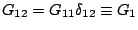
The equations can be considerably simplified if the hybridization $\Delta$ is diagonal and the Coulomb repulsion is of the form $U_{\alpha \b }n_\alpha n_\b$. In this case, propagators in the above equations are also diagonal, i.e., $G_{12}=G_{11}\delta_{12}\equiv G_{1}$ and the two particle-hole channels do not mix anymore and can be separately summed up. The two ladders become a simple geometric series and can be explicitely inserted into self-energy expression

$$\Sigma^{pp}_{\alpha }(i\omega )=T\sum_{\b }U_{\alpha \b }\sum_{i\... ..._{\alpha \b }(i\Omega )}-U_{\alpha \b }\chi^{pp}_{\alpha \b }(i\Omega ) \right]$$ (6)

$$\Sigma^{ph}_{\alpha }(i\omega )=T\sum_{\b }U_{\alpha \b }\sum_{i\... ..._{\alpha \b }(i\Omega )}-U_{\alpha \b }\chi^{ph}_{\alpha \b }(i\Omega ) \right]$$ (7)

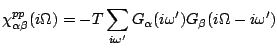
where the simplified polarisation diagrams are

$$\chi^{pp}_{\alpha \b }(i\Omega )= -T\sum_{i\omega ^\prime}G_{\alpha }(i\omega ^\prime)G_{\b }(i\Omega -i\omega ^\prime)$$ (8)

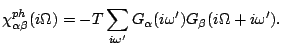$$\chi^{ph}_{\alpha \b }(i\Omega )=-T\sum_{i\omega ^\prime}G_{\alpha }(i\omega ^\prime)G_{\b }(i\Omega +i\omega ^\prime).$$ (9)

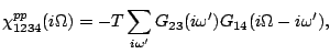
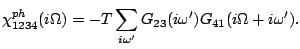
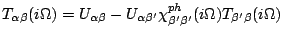
The third GW channel can also be analytically summed up for the SU(N) case, but if the crystal field splitting is assumed, one still needs to solve a matrix equation

$$T_{\alpha \b }(i\Omega ) = U_{\alpha \b }-U_{\alpha \b ^\prime} \chi^{ph}_{\beta^\prime\beta^\prime}(i\Omega )T_{\beta^\prime\beta}(i\Omega )$$ (10)

to obtain the self-energy of this channel

$$\Sigma^{gw}_{\alpha }(i\omega )=-T\sum_{i\Omega }G_{\alpha }(i\om... ...\alpha }(i\Omega )+\sum_\b U_{\alpha \b }^2\chi^{ph}_{\b\b }(i\Omega ) \right].$$ (11)

In the SU(N) case, the summation can be performed and the result is

$$\Sigma^{gw}_{\alpha }(i\omega )=-T\sum_{i\Omega }G(i\omega +i\Ome... ...i^{ph}(i\Omega)}-\frac{U}{1-U\chi^{ph}(i\Omega)}+N U\chi^{ph}(i\Omega)\right].$$ (12)

Somethimes it is more convenient to work on real axis and thus avoid the problem of analytic continuation. The price one pays is that the functions on real axis have more structure to resolve and the equidistant mesh is in many cases too expensive. Therefore, it is desired to work with nonequidistant meshes on real axes with more points around zero frequency where Fermi function drops quickly and most of sensitive structure is located. 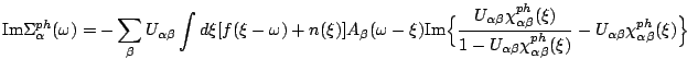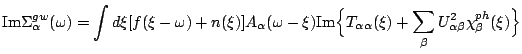The FLEX equations can be analytically continued to real axes by the standard contour integration and the results is

$$\mathrm{Im}\{\chi^{ph}_{\alpha \b }(\Omega )\}=\pi\int d\xi[f(\xi-\Omega )-f(\xi)]A_{\alpha }(\xi)A_{\b }(\xi-\Omega )$$ (13)

$$\mathrm{Im}\{\chi^{pp}_{\alpha \b }(\Omega )\}=\pi\int d\xi[f(\xi-\Omega )-f(\xi)]A_{\alpha }(\xi)A_{\b }(\Omega -\xi)$$ (14)

$$T_{\alpha \b }(\Omega ) = U_{\alpha \b }-U_{\alpha \b ^\prime} \chi^{ph}_{\beta^\prime\beta^\prime}(\Omega )T_{\beta^\prime\beta}(\Omega )$$ (15)

$$\mathrm{Im}\Sigma^{ph}_{\alpha }(\omega )=-\sum_{\b }U_{\alpha \b... ... }\chi^{ph}_{\alpha \b }(\xi)}-U_{\alpha \b }\chi^{ph}_{\alpha \b }(\xi) \Big\}$$ (16)

$$\mathrm{Im}\Sigma^{pp}_{\alpha }(\omega )=-\sum_{\b }U_{\alpha \b... ... }\chi^{pp}_{\alpha \b }(\xi)}-U_{\alpha \b }\chi^{pp}_{\alpha \b }(\xi) \Big\}$$ (17)

$$\mathrm{Im}\Sigma^{gw}_{\alpha }(\omega )=\int d\xi[f(\xi-\omega ... ...Big\{T_{\alpha \alpha }(\xi)+\sum_\b U_{\alpha \b }^2 \chi^{ph}_\b (\xi) \Big\}$$ (18)

In the SU(N) case, the last contribution can again be simplified to

$$\mathrm{Im}\Sigma^{gw}_{\alpha }(\omega )=-\int d\xi[f(\xi-\omega... ...{Im}\Big\{ \frac{U\chi}{1-U\chi}+\frac{(N-1)U\chi}{1+(N-1)U\chi}-N U\chi \Big\}$$ (19)