Computation LDA band structure
We use LDA calculations in order in addition to the total energy, bands, optical properties in non-interacting limit, to extract the Hamiltonian and the overlap matrixes as well as some other auxiliary arrays containing additional information about structure of a studied material to be used in DMFT calculations.
We have chosen the Liner Muffin-Tin Orbitals (LMTO) in Atomic Sphere Approximation (ASA) and Full Potential (FP) program written by S. Savrassov. Below we provide an example how to run the program using LaTiO3 compound (paramagnetic, undistorted). Extended manual of the program as well as graphical interface to is one can find on web page of S. Savrasov.
We used LaTiO3 in our calculations as it has a simple band structure with three degenerate t2g bands, which accommodate one electron (in the undistorted case). And those three bands can be easily described by three-fold degenerate Hubbard model which one could use to obtain the self-energy.
Suppose you have compiled the program which is now ready to run. We tested and run program on the following platforms: IBM AIX, ALPHA OSF, Linux RedHat and SuSE, and Windows. We used available for those platform commercial compilers. Under Linux we used PGI and FREE Intel compiler. Typical input into the program is the following (run file):
/home/user/LMTO/main <<!
Latio3
ini+str+scs
scf
!
The first line is the full path to the executable. The second one is the name of the compound to run. All files in directory should have this name. The files have different extension, which describe their meaning.
The third line just attributes to those extensions: ini is the control file where majority of physical parameters are described, str is the structural file where positions of atoms along with other structural information is located. These two files are minimum information, which is necessary to start the program. Actually if one starts from scratch as an initial guess one uses atomic potentials for atoms which constitute the compound. Information about atomic potentials is located in separate directory “atomdata”. If one run already program and has scs (self-consistency file) then the program will start using this file. So, the third line describes input files for the program. The fourth line is the output line, one tells to the program what should be calculated. In the example above we ask for the self-consistency run: it should be obtained a self-consistent solution for a material studied. After the self-consistent solution obtained one can ask to compute other properties. But! FMM: Before to proceed one should copy (rename) scf file onto scs. As scs file is the starting file for any further calculations and it is quite reasonable to use the self-consistent solution for properties to study. Other options of the fourth line are: fat (“fat” bands calculations), dos (density of states), opt (optical properties). If one wants take into account correlation using LDA+U method then one more input file is needed, which is hub (HUBbard) file (the third line) where correlations and their strength are described. (<<! ... ! is the usual Unix stuff to make interactive input in batch file).
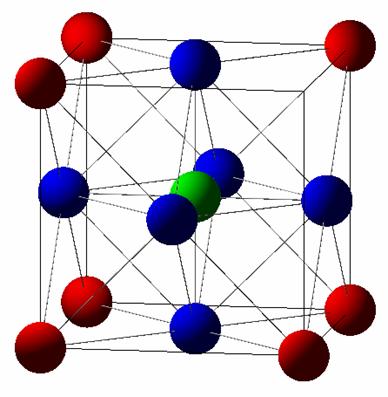
So, we need 2 files: ini and str. We will not discuss now how to prepare ini file as a very good description of the file can be found in help files to the program or on the S. Savrasov webpage. In addition each line in the ini file is provided comment. One can easily understand what is what. To prepare str file is a little bit more tricky especially if one dials with 20 and more atoms but in the case of 5 atoms the situation is quite simple. And it also depends on the way to put structure information used in the program. There are two basic approaches to start first principles LDA calculations a) to put a group number and positions of those atoms in the table as they are b) approach which is to find the corresponding group symmetry once provided with positions of atoms. We used in our program the second approach and put into structure file the following atomic positions. The positions should be “unique” in the sense that coordinates of the atoms from the structural file couldn’t be obtained using basic orthorhombic shifts (a,b,c). Using these unique positions program will generate full cell automatically.
Below we present
results obtained for simple cubic lattice using two methods: LMTO-ASA and
LMTO-FP. The only line which should be changed in ini
file is FulPot=ASA or PLW.
We used the following control (ini) and structure (str) files:
|
INI |
STR |
|
<FILE=INIFILE,INPUT=MODERN,TRACE=FALSE> <SECTION=HEAD> Title = Bands 01 <SECTION=CTRL> LMTO = Screened FulPot = ASA <SECTION=EXCH> LDA = Vosko GGA = none <SECTION=ITER> Niter1 = 30 <SECTION=MAIN> nAtom
= 5 nSort
= 3 Is(J = 1 2 3 3 3 Par0 = 7.4 <SECTION=SORT> Name = La Znuc
= 57.0 <SECTION=SORT> Name = Ti Znuc
= 22.0 <SECTION=SORT> Name = O Znuc
= 8.0 <SECTION=FFTS> nDiv(:) = 10,10,10 |
<FILE=STRFILE,INPUT=MODERN> <SECTION=CTRS> nAtom
= 5 BtoA = 1.0 CtoA = 1.0 <SECTION=TRAN> 1.0, 0.0, 0.0 0.0, 1.0, 0.0 0.0, 0.0, 1.0 <SECTION=BASS> 0, 0 ,
0 !La 1/2 , 1/2, 1/2
!Ti 1/2 , 1/2, 0
!O 1/2 , 0,
1/2 !O 0, 1/2, 1/2 !O |
|
|
|
Results (ASA):
|
Structure: |
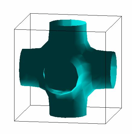
Fermi Surface: |
|
|
|
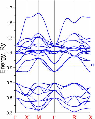
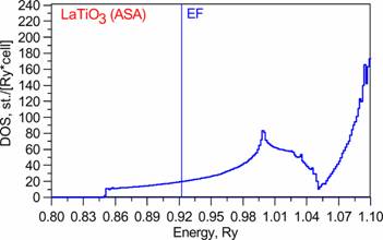
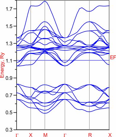
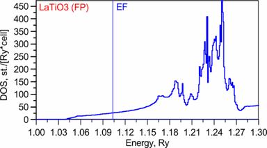
Below we present band-structure and DOS of the studied material. From ASA band structure one sees that 3band cross the Fermi level. They are Ti 3d t2g bands. Which are pretty good separated from other bands (at least in ASA). More detailed description of band-structure subtleties one can find in before mentioned paper.
|
Band-structure: |
DOS: |
|
|
|
|
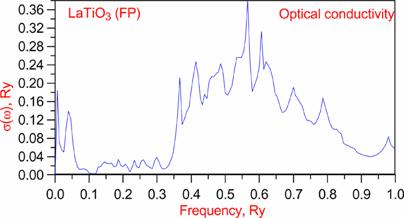
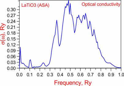
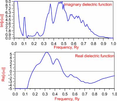
Optics: |
w=0.30875 |
|
|
|
![]()
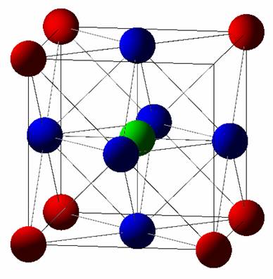
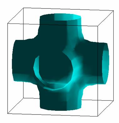
Results (Full Potential):
|
Structure: |
Fermi Surface: |
||
|
|
|
||
|
Band-structure: |
DOS: |
||
|
|
|
||
|
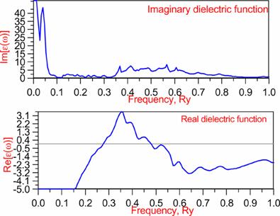
Optics: |
w=0.30038 |
|
|
|