Details of NCA evaluation

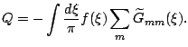
The NCA diagrams correspond to the following analytic expression for the pseudoparticle self-energy

$$\Sigma_{mn}(i\omega) = \sum_{\alpha \b ,m^{\prime}n^{\prime}}\left[ F^{\b }_{mm^{\prime}... ...n}\int d\xi f(\xi) A_{\alpha \b }(\xi)G_{m^\prime n^\prime}(i\omega+\xi)\right.$$

$$\left.\qquad+ (F^{\b\dagger})_{mm^{\prime}}F^{\alpha }_{n^\prime n}\int d\xi f(-\xi) A_{\b\alpha }(\xi)G_{m^\prime n^\prime}(i\omega-\xi)\right].$$ (1)

where $F_{nm}^{\alpha }=\langle n\vert d_{\alpha }\vert m\rangle$ are matrix elements of destruction operator of a local electron, $G_{nm}$ are pseudoparticle Green's functions and $\Sigma_{mn}$ are corresponding self-energies, i.e.,

$$(G^{-1})_{mn}=\omega-E_{mn}-\lambda-\Sigma_{mn}$$ (2)

and $E_{mn}$ is the energy of the local state in the atomic limit. The bath spectral functions $A_{\alpha\beta}$ is related to the hybridization function $\Delta$ by the following identity $A_{\alpha \b }=-1/(2\pi i)[\Delta_{\alpha \b }(\omega+i0^+)-\Delta_{\alpha \b }(\omega-i0^+)]$.

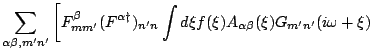
To simplify the equations, we will write them in terms of spectral quantities instead of Green's functions. Let us define

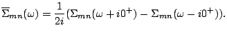
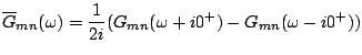$$\overline{G}_{mn}(\omega)=\frac{1}{2 i} (G_{mn}(\omega+i0^+)-G_{mn}(\omega-i0^+))$$ (3)

$$\overline{\Sigma}_{mn}(\omega)=\frac{1}{2 i} (\Sigma_{mn}(\omega+i0^+)-\Sigma_{mn}(\omega-i0^+)).$$ (4)

The quantities with hat are obviously hermitian $\overline{\Sigma}^\dagger=\overline{\Sigma}$ and the spectral function of the Green's function is proportional to the spectral density $\rho$, i.e., $\rho=-\overline{G}/\pi$.

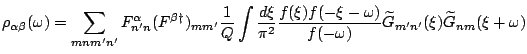
With the above definitions, the NCA equations simplify to

$$\overline{\Sigma}_{mn}(\omega)= \sum_{\alpha \b ,m^{\prime}n^{\pr... ...F^{\b\dagger})_{mm^{\prime}}F^{\alpha }_{n^\prime n} A_{\b\alpha }(-\xi)\right]$$ (5)

The local electron Green's function within NCA approximation is given by

$$G_{\alpha \b }(i\omega)=-\sum_{mnm^\prime n^\prime}F^{\alpha }_{n... ...}(\xi+i\omega)-G_{m^\prime n^\prime}(\xi-i\omega)\overline{G}_{nm}(\xi)\right],$$ (6)

where the grand canonical expectation value of the charge $Q$ (or equivalently the partition function of the impurity) is given by

$$Q=-\int\frac{d\xi}{\pi}\exp(-\beta\xi)\sum_m \overline{G}_{mm}(\xi).$$ (7)

We will again write the equation for the spectral function rather than the Green's function. The local electron spectral function $\rho$ becomes

$${\rho}_{\alpha \b }(\omega)=\sum_{mnm^\prime n^\prime}F^{\alpha }... ...eta\omega}] \overline{G}_{m^\prime n^\prime}(\xi)\overline{G}_{nm}(\xi+\omega)$$ (8)

The system of equations Eq. (2), (5), (8) and (7) is thus closed.

Let me pause here for a moment and show that the equations are invariant with respect to the shift of frequency in the pseudo particle quantities due to local gauge symmetry, therefore $\lambda$ that appears in the definition of the pseudo Green's functions can be an arbitrary number. In numerical evaluation, we use this to our advantage and choose zero frequency at the point where pseudo particle spectral functions diverge. First, we want to show that shift of frequency arguments of all pseudo-particle quantities by $\delta\lambda$ does not affect the equations provided that $\lambda$ also changes to $\lambda\rightarrow\lambda+\delta\lambda$

$$[G^{-1}(\omega+\delta\lambda)]_{mn}=\omega-E_{mn}-\lambda-\Sigma_{mn}(\omega+\delta\lambda)$$ (9)

$$\overline{\Sigma}_{mn}(\omega+\delta\lambda)= \sum_{\alpha \b ,m^... ...F^{\b\dagger})_{mm^{\prime}}F^{\alpha }_{n^\prime n} A_{\b\alpha }(-\xi)\right]$$ (10)

$${\rho}_{\alpha \b }(\omega)=\frac{\sum_{mnm^\prime n^\prime}F^{\a... ...(-\frac{d\xi}{\pi})\exp(-\beta\xi)\sum_m \overline{G}_{mm}(\xi+\delta\lambda)}.$$ (11)

The above equations are obviously unchanged. Notice that the physical quantities like the local spectral function and the baths spectral function are not affected by the shift. The auxiliary charge $Q$, however, changes $Q\rightarrow Q\exp(-\beta\delta\lambda)$.

In numerical evaluation, we can either fix $\lambda$ and calculate $Q$, or alternatively, fix $Q$ and calculate $\lambda$ at each iteration. The goal is to resolve the structure of the pseudo-particle functions and therefore it is best to choose the zero frequency at the point where the pseudo-quantities have a threshold (they diverge at zero temperature). In the program, user can fix $Q$ to an arbitrary number and the corresponding $\lambda$, which is just the impurity free energy, is calculated. This guarantees that in zero temperature limit the threshold point is at zero frequency. For small number of local states, like for the one band model, the choice $Q=1$ is best. When the number of bands grows, $Q$ should grow as well. A good choice is $Q\approx N_{all}$ where $N_{all}$ is the number of all local states.

The above NCA equations are still numerically intractable because of exponential factors appearing in Eq. (7) and (8). As we mentioned, the pseudo-quantities have a threshold, i.e., they exponentially vanish below a certain frequency (which is zero frequency if $Q$ is a fixed constant). However, the exponential tails obviously enter the equation Eq. (7) and need to be calculated. The problem can be circumvented by defining new quantities that coincide with the original quantities above the threshold, but are nonzero also below the threshold and carry the information needed below the threshold. We will use the tilde sign for those new quantities

$$\widetilde{G}(\omega)= \overline{G}(\omega)/f(-\omega)$$ (12)

$$\widetilde{\Sigma}(\omega) = \overline{\Sigma}(\omega)/f(-\omega).$$ (13)

Substituting the tilde quantities in the Eq. (5), (7) and (8), we obtain

$$\widetilde{\Sigma}_{mn}(\omega)= \sum_{\alpha \b ,m^{\prime}n^{\p... ...F^{\b\dagger})_{mm^{\prime}}F^{\alpha }_{n^\prime n} A_{\b\alpha }(-\xi)\right]$$ (14)

$${\rho}_{\alpha \b }(\omega)=\sum_{mnm^\prime n^\prime}F^{\alpha }... ...(-\omega)} \widetilde{G}_{m^\prime n^\prime}(\xi)\widetilde{G}_{nm}(\xi+\omega)$$ (15)

$$Q=-\int\frac{d\xi}{\pi} f(\xi)\sum_m \widetilde{G}_{mm}(\xi).$$ (16)

The system of NCA equations Eq. (14), (15) and (16) is numerically more tractable and free of diverging exponential factors. Namely, the combination of Fermi functions ${f(\xi)f(-\xi-\omega)}/{f(-\omega)}$ is always less than unity and can be very accurately calculated by realizing that

$$\frac{f(\xi)f(-\xi-\omega)}{f(-\omega)}=\frac{f(-\xi)f(\xi+\omega)}{f(\omega)}=f(\xi)f(-\xi-\omega)+f(-\xi)f(\xi+\omega),$$

is just a window function.