A note on calculating convolutions

Most of the Green's functions and specially Fermi function at low temperature are very steep or peaked at certain points (usualy around zero). The use of equidistant mesh is therefore impractical and time consuming, rather a non-equidistant mesh is desired. We usualy use logarithmic mesh at low frequency and tanges mesh at high frequnecies to resolve almost any function with less than 300 points. The prices one needs to pay using nonequidistant mesh is that a convolution like

$$C(z)=\int g(x)f(x-z)dx$$ (17)

is much harder to calculate since it is not resolved on the first mesh neither on the second. Suppose that $g(x)$ is defined on a certain mesh $\{x_i\}$ where it is resolved $g(x_i)\equiv g_i$ and function $f(y)$ is defined on another mesh $\{y_i\}$, i.e., $f(y_i)\equiv f_i$, the convolution can be safely calculated on the union of both mashes $\{x_i,y_j+z\}$. One of the meshes should be shifted for $z$, thus for each outside frequency a different union of the two meshes should be formed and only then the convolution can be safely evaluated. This is very time consuming and seldom done in practice.

We have two strategies to circumvent the problem. If one knows that both functions are peaked around certain point, lets suppose zero frequency, we can form a two-dimensional mesh (somewhere in the outside loop such that it is heavily reused) in which the first mesh $\{x_i\}$ is superposed with couple of points around zero frequency from mesh $\{y_j\}$.

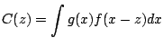
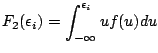
However, when a certain function needs to be convolved with many other functions (typical case is NCA with many nonequivalent pseudo-particles), one can use a trick. With the help of two additional precalculated functions, the integral and first moment

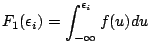$$F_1(\epsilon_i) = \int_{-\infty}^{\epsilon_i}f(u)du$$ (18)

$$F_2(\epsilon_i) = \int_{-\infty}^{\epsilon_i}u f(u)du$$ (19)

one can calculate the convolution without building a new inside mesh. Lets use the mesh $\{x_i\}$ which resolves function $g$. Then, in the spirit of trapezoid rule, we can lineraly interpolate $g$ between the points

$$C(z)=\sum_i \int_{x_i}^{x_{i+1}} \left[g_i+\frac{g_{i+1}-g_i}{x_{i+1}-x_i}(x-x_i)\right]f(x-z)dx.$$ (20)

This integral can be expressed by the above defined functions. To show that, let us rewrite the convolution and expressed it by the new function $\langle f\rangle_i$ which is defined on the same mesh as $g$ and with which the covolution is a simple scalar product

$$C(z)=\sum_i g_i\left[ \int_{x_i-z}^{x_{i+1}-z}\frac{x_{i+1}-z-u}... ...{i-1}}{x_{i}-x_{i-1}}f(u)du \right]\equiv \sum_i g_i \langle f\rangle_i dh_i .$$ (21)

Thus $\langle f\rangle_i$ is

$$\langle f\rangle_i= \frac{2}{x_{i+1}-x_{i-1}}\left[ \int_{x_i-z}^... ...(u)du + \int_{x_{i-1}-z}^{x_i-z}\frac{z+u-x_{i-1}}{x_{i}-x_{i-1}}f(u)du \right]$$ (22)

$$= \frac{2}{x_{i+1}-x_{i-1}}\left[ \frac{(x_{i+1}-z)[F_1(x_{i+1}-z)-F_1(x_i-z)]-F_2(x_{i+1}-z)+F_2(x_i-z)}{x_{i+1}-x_i}- \right.$$ (23)

$$\left.- \frac{(x_{i-1}-z)[F_1(x_i-z)-F_1(x_{i-1}-z)]-F_2(x_i-z)+F_2(x_{i-1}-z)]}{x_{i}-x_{i-1}} \right]$$ (24)

This method is specially suitable if function $f$ needs to be convolved with many different functions that live on the same mesh $\{x_i\}$ because the function $\langle f\rangle_i$ can be calculated ones and reused many times. This is the case of NCA with many nonequivalent local states. The method is also crucial for implementing higher-order vertex correction to NCA. The implementation can be found in the header file average.h.